EGC: a simple case study

Abstract. This blog article investigates Exact Geometric Computation libraries in general and CORE and LEDA in particular. The starting point is a simple toy problem of testing whether the sum of numbers equals zero and the question whether the way we build the sum significantly influences the runtime and memory costs. The results obtained question the practical implications of complexity analysis w.r.t. the RealRAM model and motivate optimization strategies for EGC libraries. This article also sheds light on runtime, memory and correctness issues that were raised by benchmarks.

Parts of the results discussed here were presented in a talk “Implementing Geometric Algorithms for Real-World Applications With and Without EGC-Support” given at the CGWeek 2013.

Preliminaries

Motivation. Exact Geometric Computation (EGC) or Exact Arithmetics is a technology to overcome the notorious difficulties with numerical stability in implementations of geometric algorithms caused by finite precision floating-point arithmetic, as it is provided by the widespread IEEE-754 floating-point units.

In contrast to, say, linear algebra problems, where numerical instability essentially affects the accuracy of the output (Eigen value, determinant, etc.), in geometric codes the control flow of programs depends on geometric (i.e., numerical) decisions. Consequently inaccuracies easily lead to an inconsistent perception of geometric settings, which often causes programs to crash. The goal behind EGC is to have guaranteed correct results when comparing an expression “x” against zero, say “x = 0” or “x < 0” or “x > 0”.

A brief introduction to EGC. This goal is achieved by maintaining for “x” the entire expression tree.¹ This allows you to evaluate the expression “x” with any precision you like using, say, the arbitrary precision library MPFR. As you can bound the numerical errors of sqrt, +, *, etc. you can deviate a lower bound L and upper bound U for the precise value behind “x” depending on the precision. The difference U-L tends to zero as the precision increases. Assume that “x” is indeed negative, then you could iteratively double the precision and at some point U will become negative, too: you end up with L ≤ x ≤ U < 0. Hence, you can guarantee that x is negative.

But what if x is actually zero? Then, no matter what precision you choose you are stick to L ≤ 0 ≤ U and it seems as if you cannot tell the sign of x as long as U-L > 0. Here comes the concept of root bounds into play: If U-L goes below the so-called root bound then you can still be certain that x is actually zero. Figuratively speaking, even if x = (1 + sqrt(2))² - 2*sqrt(2) - 3 evaluates to -0.00…001 you know that it is precisely zero, if there is a sufficient number of zero digits.

Of course, maintaining expression trees and iteratively evaluating the nodes with “software floating-point numbers” by means of MPFR comes along with high costs. These costs are greatly reduced by so-called floating-point filters. The idea is to do the computation in machine precision a-priori and keeping track of the errors. And in many cases the 53 bits for the mantissa of IEEE double-precision values suffice to guarantee correctness of comparisons. In case it cannot be guaranteed, the big machinery is applied.

There are two major libraries that provide EGC to real-world applications: CORE and LEDA. Both are written in C++ and provide a datatype for real numbers that can be used as a drop-in replacement of the built-in machine ‘double’ by preprocessor directives. They also constitute the (exact) arithmetic foundation of the CGAL library.

A simple experiment

Consider a toy problem with geometric flavor: We want to test whether the center of gravity of finitely many points is at the origin. We can break this down to the question whether the sum of finitely many real numbers in an array is zero. For this reason we generate an array with random² numbers k and -k.

bool test(unsigned N) {
    vector<Real> arr;
    for (unsigned i = 0; i < N; ++i) {
        int x = rand();
        arr.push_back(Real(x));
        arr.push_back(-Real(x));
    }
    std::random_shuffle(arr.begin(), arr.end());
    return Real(0) == buildsum(arr.begin(), arr.end());
}

The straight-forward C++ way of implementing buildsum would be something like this:

Real buildsum(vector<Real>::iterator beg, vector<Real>::iterator end) {
    Real sum(0);
    for (vector<Real>::iterator it = beg; it != end; ++it)
        sum += *it;
    return sum;
}

So this is a simple O(n) time and O(1) space algorithm. Well, to be precise, these complexities apply to the RealRAM model. We simply loop over the input array and accumulate the sum in a local variable. But recall that in the background expression trees are maintained. It seems justified to assume that high expression trees correspond to a high demand for precision to have guaranteed correct comparisons. Hence, it is probably better to build the sum such that the expression tree is balanced, and maybe even better if the bottom level is filled from one side such that the leaf nodes are clustered to the same sub-trees:

Real buildsum_balanced(vector<Real>::iterator beg, vector<Real>::iterator end) {
    if (beg + 1 == end)
        return *beg;
    unsigned up = ceil_power2(end-beg);
    vector<Real>::iterator mid = beg + up/2;
    return buildsum_balanced(beg, mid) + buildsum_balanced(mid, end);
}

Experiment 1

Below you see a runtime plot with six different configurations: CORE-2.1³ vs. LEDA-6.3 (free edition), with and without floating-point filters⁴, with and without balancing the expression tree. For the right plot I added the small number 2^-65 to the array before shuffling it and test() checks whether the sum is non-zero. So we expect in any case that test() returns true. If you click on the plot a full-size figure is shown that also contains RSS and stack memory consumption and the statistics for buildsum().⁵

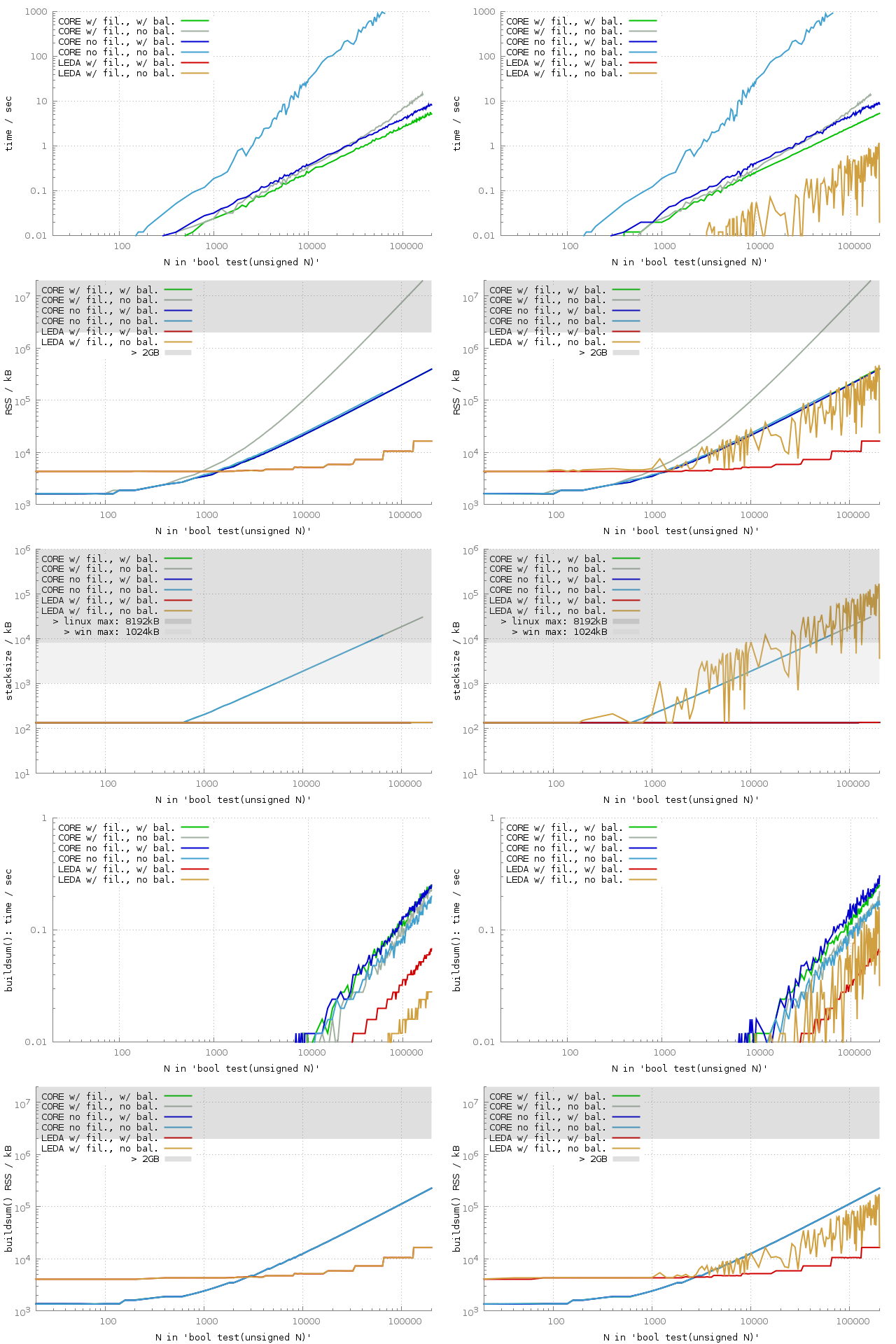
A few comments:

• The benchmarks were performed on Debian Linux using a Six-Core AMD Opteron(tm) Processor 2431 clocked at 2.4 GHz and 64 GB main memory. Three benchmark processes were launched in parallel. Each run was limited to 1000 seconds runtime, 20 GB RSS and 1 GB stack size.

• CORE/unbalanced without filters has an approx. O(n²) time consumption. Using valgrind’s callgrind tool and N=4000 the reason turns out to be the following:

  • 98 % of the time is consumed by ExprRepT::refine(), which is called recursively called in total 990 times when determining the sign of the sum expression.
  • Within refine(), 91 % of the time is consumed by get_constructive_bound(), which again mostly consists of get_Deg(). Both are again called 990 times in total.
  • Every call of get_Deg(), however, calls compute_Deg(long) and rootBd_init() recursively again, and hence about 9.6 million times in total. This causes the O(n²) runtime.

• CORE/unbalanced with filters lead a shift of the O(n²) runtime issue to higher N. That is, we see that the runtime graph stops the linear behavior at roughly N=60000.

  The more severe issue, however, is the O(n²) memory consumption in the unbalanced, filtered case. With N=50000 roughly 2 GB of memory are allocated, which constitutes a hard limit⁶ on many 32-bit systems.

  Using valgrind’s massif⁷ tool and N=40000 we can conclude the following:

  • AddSubRepT::compute_a_approx(long precision) indirectly allocates 1.1 GB of memory, with a RSS of 1.4 GB. AddSubRepT::compute_a_approx() itself calls BigFloat::set_prec(), which then calls mpfr_set_prec(), which allocates the 1.1 GB.

  • The first call of refine() calls AddSubRepT::compute_a_approx(), which calls itself recursively in total 79999 times. But the precision argument to the recursive call is increased by two for each child. Hence, in the unbalanced case, the arithmetic sum of precision among all nodes is in O(n²), causing a quadratic memory consumption.

    In the unfiltered case refine() is called more often because the signs of the subtrees are unknown due to the missing filters. Hence, sub-trees often already have suitable approximate values by previous refine() calls and is_approx_needed() returns false. This leads to shorter recursive runs of AddSubRepT::compute_a_approx(long) and hence smaller precisions.

• In the left plot we do not see LEDA at all: LEDA has virtually zero runtime.⁸ In the right plot LEDA/unbalanced does show up, but with quite unstable runtimes. If we consider the expression tree, we see a degenerated list and 2^-65 is located somewhere. If it is at the bottom of the tree (i.e., at the front in the array) then runtime is high. If its at the top of the tree (i.e., at the back in the array), runtime is virtually zero, as in the left plot.

  The reason might be that from bottom to top the filters work well until 2^-65 is encountered and for the left plot the sum could be precisely expressed by machine double. If filters stop to work, arbitrary precision numbers need to be employed. Indeed, the higher runtime also comes along with higher memory consumption, both for heap and stack, both for testing the sum and for constructing the expression. Also, if we add 2^-65 and -2^-65 to the array then LEDA has an observable runtime also for the zero-test.

  In the balanced case 2^-65 is just one among 2N + 1 leafs of the tree.

• For CORE with and without filters we observe quite a large stack size in the unbalanced cases. The default maximum stack size of 1024 kB for executables produced by Visual Studio is reached for N=5000. Interestingly, LEDA was in the unbalanced case of the non-zero test even more demanding and used roughly a factor of 4 more stack memory.

  For our tests under Linux we increased the maximum stack size from the default 8192 kB to 1 GB.

Experiment 2

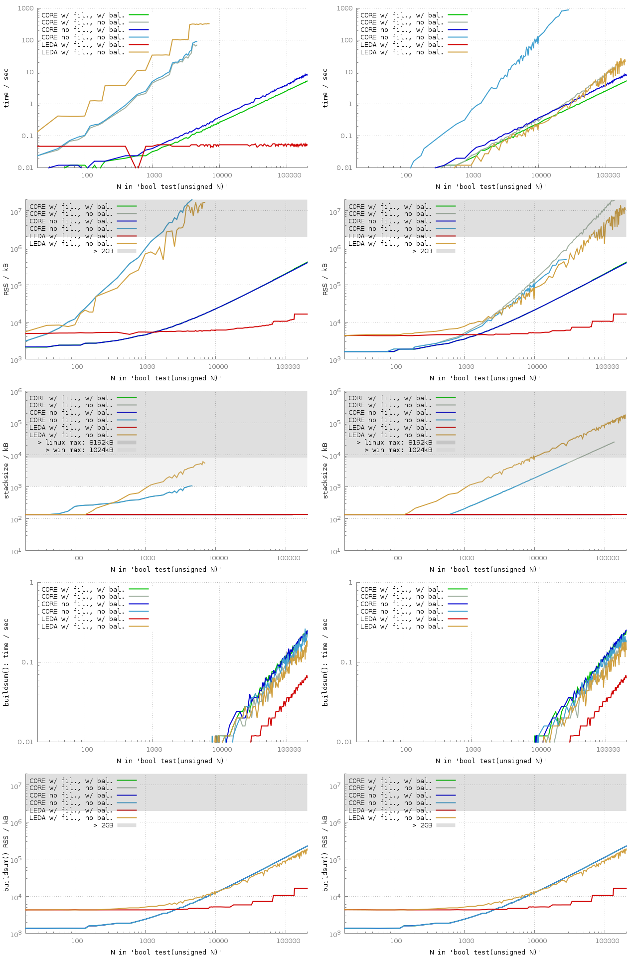
For the following plot, we put more stress on the floating-point filters by adding five sqrt(2) and -sqrt(2) expressions to the array in order to retrieve observable runtimes for LEDA. (Adding five such pairs instead of one avoids the jumpy runtime, as we have seen it in the non-zero LEDA test.)

• As expected, the impact of filters becomes rather negligible in the zero test, especially in the unbalanced case. Hence, we observe in all unbalanced cases approximately an O(n²) runtime complexity.

  In the balanced case almost all subtrees are still rational and could be even precisely evaluated by machine doubles. LEDA is obviously able to exploit this fact best. CORE at least is able to take advantage of the filters to some extent, speeding up by a factor of 2.

• In the non-zero test, the 2^-65 summand prevented filters in the previous experiment, too. Hence the outcome is quite similar as before, with the additional constant penalty of the sqrt(2) expressions.

• To the balanced cases the additional sqrt(2) summands have a negligible impact.

• The ten additional sqrt(2) summands caused the memory consumption of all unbalanced cases, in the zero and non-zero test, to grow to O(n²). Filters have virtually no impact on memory consumption for CORE. Only in the non-zero test in the unbalanced case, filters cause a slightly higher memory consumption.

• Concerning the stack size, we observe that LEDA is even more demanding than CORE. In the zero test, LEDA crossed the default max size of 1 MB under Windows at N=1000. In the non-zero test, LEDA crosses the 100 MB stacksize at N=100000.

Experiment 3

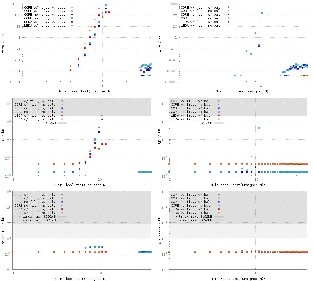
As only a few sqrt() expressions appear to have a serious impact on the runtime of our experiments, we also ran an experiment where we consider sums of sqrt(k) and -sqrt(k) expressions for random numbers k.

• Every experiment was done ten times with different seeds to rand(). The above figure contains the arithmetic means of the results. However, especially for LEDA/balanced, the runtime is quite unpredictable and ranges within 5 orders of magnitude: for N=9 the runtime ranged from 16 ms to 179 s. For CORE the results are more deterministic; only in the balanced case at N=9, the maximum runtime is about a factor 7 higher then the minimum runtime.

• For all configurations in the zero test, the runtime is somewhere between O(n⁸) and O(n¹⁰). The runtime of each experiment has been limited to 1000 sec and no test finished within this constraint for N ≥ 13.⁹ (The outliers to the right are discussed below.)

  In fact, the following CORE expression takes 138 seconds to return true:

  // simplesum.cpp
  Expr(0) ==
          + sqrt(Expr(1804289383))
          + sqrt(Expr(846930886))
          + sqrt(Expr(1681692777))
          + sqrt(Expr(1714636915))
          + sqrt(Expr(1957747793))
          + sqrt(Expr(424238335))
          + sqrt(Expr(719885386))
          + sqrt(Expr(1649760492))
          + sqrt(Expr(596516649))
          + sqrt(Expr(1189641421))
  
          - sqrt(Expr(1804289383))
          - sqrt(Expr(846930886))
          - sqrt(Expr(1681692777))
          - sqrt(Expr(1714636915))
          - sqrt(Expr(1957747793))
          - sqrt(Expr(424238335))
          - sqrt(Expr(719885386))
          - sqrt(Expr(1649760492))
          - sqrt(Expr(596516649))
          - sqrt(Expr(1189641421))
  

  The tutorial that is shipped with the CORE library contains the following warning:

  Expr s = 0;
  for (int i=1; i<=100; i++) s += sqrt(Expr(i));
  

  You can easily evaluate this number s, for example. But you will encounter trouble when trying to compare to such numbers that happen to be identical.

• CORE returns the correct result true for N≥30 within milliseconds, which is surprising given the results for N≤10. One first suspects that the cutoff-bound is reached. However, turning on debugging capabilities does not confirm this and no diagnostics file is created. Nevertheless, the exact arithmetics machinery does not work. That is, the non-zero test fails.

  In particular, the following code silently fails and returns false:

  // simplesum-fail.cpp
  Expr(0) !=
          sqrt(Expr(1804289383))
          + sqrt(Expr(846930886))     + sqrt(Expr(1681692777))
          + sqrt(Expr(1714636915))    + sqrt(Expr(1957747793))
          + sqrt(Expr(424238335))     + sqrt(Expr(719885386))
          + sqrt(Expr(1649760492))    + sqrt(Expr(596516649))
          + sqrt(Expr(1189641421))    + sqrt(Expr(1025202362))
          + sqrt(Expr(1350490027))    + sqrt(Expr(783368690))
          + sqrt(Expr(1102520059))    + sqrt(Expr(2044897763))
          + sqrt(Expr(1967513926))    + sqrt(Expr(1365180540))
          + sqrt(Expr(1540383426))    + sqrt(Expr(304089172))
          + sqrt(Expr(1303455736))    + sqrt(Expr(35005211))
          + sqrt(Expr(521595368))     + sqrt(Expr(294702567))
          + sqrt(Expr(1726956429))    + sqrt(Expr(336465782))
          + sqrt(Expr(861021530))     + sqrt(Expr(278722862))
          + sqrt(Expr(233665123))     + sqrt(Expr(2145174067))
          + Expr("0.00000000000000001")
          - sqrt(Expr(1804289383))
          - sqrt(Expr(846930886))     - sqrt(Expr(1681692777))
          - sqrt(Expr(1714636915))    - sqrt(Expr(1957747793))
          - sqrt(Expr(424238335))     - sqrt(Expr(719885386))
          - sqrt(Expr(1649760492))    - sqrt(Expr(596516649))
          - sqrt(Expr(1189641421))    - sqrt(Expr(1025202362))
          - sqrt(Expr(1350490027))    - sqrt(Expr(783368690))
          - sqrt(Expr(1102520059))    - sqrt(Expr(2044897763))
          - sqrt(Expr(1967513926))    - sqrt(Expr(1365180540))
          - sqrt(Expr(1540383426))    - sqrt(Expr(304089172))
          - sqrt(Expr(1303455736))    - sqrt(Expr(35005211))
          - sqrt(Expr(521595368))     - sqrt(Expr(294702567))
          - sqrt(Expr(1726956429))    - sqrt(Expr(336465782))
          - sqrt(Expr(861021530))     - sqrt(Expr(278722862))
          - sqrt(Expr(233665123))     - sqrt(Expr(2145174067))
  

Discussion

Optimizations of expression trees. The experiments conducted demonstrate that balancing expression trees saves a significant amount of computing time and memory:

• When floating-point filters are not (or cannot be) applied, often a linear factor in time and/or space is saved.
• Beyond that, balancing expression trees sometimes actually enables the application of floating-point filters.
• Even when filters are applied, balanced trees often are by some non-negiglible constant factor faster and/or more space efficient.
• With balanced expression trees, the operating system’s default stack sizes were always sufficient.

Hence, it would be worth to investigate on- or offline balancing techniques for connected components of expression trees consisting of the same commutative operators, similar to the techniques known for binary-tree data structures. Maybe, those techniques could be applied when some threshold for the height of an expression tree is reached or when some threshold in the precision refinement is reached.

Migrating present code to EGC. When a new geometric software project is launched and EGC libraries are used, the developers better pay close attention to the expressinon trees that are build behind the scenes. Migrating a present non-trivial software project to an EGC arithmetic backend will most certainly turn out to be non-trivial.

Complexities, EGC and RealRAM. The discussion started with a simple O(n) time and O(1) space algorithm in the RealRAM model. It is clear that machine-precision floating-point arithmetic is no adequat implementation of the RealRAM model when it comes to numerical errors (and several other reasons). However, the EGC libraries do not provide an adequate implementation of the RealRAM model, too. A simple comparison of two real numbers takes O(n²) time and often O(n²) space in our naive unbalanced implementation. This fact raises the question to which extent the ordinary complexity analysis with respect to the RealRAM model is of practical significance when it comes to EGC libraries.

Code and data. The directory files/ contains a couple of files that were used to generate the above benchmarks:

• sum.cpp: the main benchmark source code.
• simplesum.cpp and simplesum-fail.cpp, as described above.
• sum-stats.sh: the shell script to run the benchmarks. It uses paralleljobs to run the jobs in parallel.
• *.sqlite: the sqlite database that contains the benchmarks results reported here.