libstick: Demonstration

The following demonstration refers to the current version 0.2 of libstick. (Version 0.1 had no concept of a simplicial_function, but incorporated it into simplicial_complex.)

From images to complexes

Persistent homology has many applications, one of them is image analysis. Consider the following image of onion cells from an epidermal peel¹. On the left we see the gray-scale image and on the right we see the image interpreted as gray-value function \(\Omega \to [0,255]\) over the rectangular image domain \(\Omega \subset \mathbb{R}^2\).

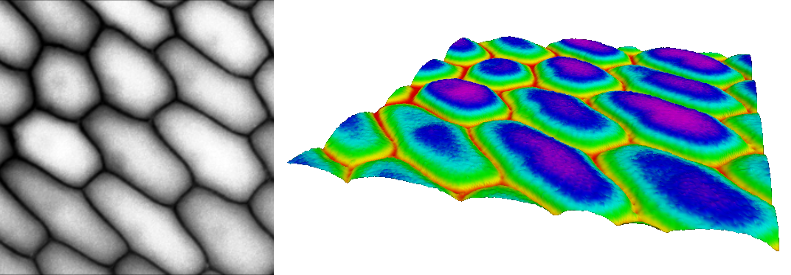
Using libstick, one can convert an image to a simplicial function on a simplicial complex in the following sense:

• Simplicial complex. Each pixel gives rise to a vertex (0-simplex) and any two pixels sharing an edge give rise to an edge (1-simplex) between the corresponding vertices representing the pixels. Each of the square faces is split into triangles by an additional 1-simplex and all the triangles are inserted as 2-simplices.

• Simplicial function. Each simplex is assigned a function value as follows: Each vertex gets assigned the gray value (between 0 and 255) of its pixel and all edges and triangles get as value the maximum value of the incident vertices.

// A simplicial complex of dimension 2, uint32_t for the indices of simplices,
// and uint8_t for the function values.
typedef libstick::simplicial_function<2, uint32_t, uinit8_t> sfunction;
typedef libstick::simplicial_complex<2, uint32_t> scomplex;
scomplex comp;
sfunction func(comp);
libstick::add_image_to_simplicialfunction(func, imagedata, width, height);

Next, one creates a monotone filtration from the simplicial complex:

scomplex::simplex_order order(comp);
func.make_order_monotonefiltration(order);

Finally, we run the matrix reduction algorithm and build the persistence diagrams. This allows us to ask, for instance, for the persistent Betti-1 number in the interval [96, 192]. The function interpret_reduction() prints information on the sequence of insertions of simplices and which cycles are born or killed due to these insertions. The function interpret_persistence() prints the points in the persistence diagram with their birth and, if existent, death times.

typedef libstick::persistence<2, uint32_t> persistence;
persistence pers(order);

pers.compute_matrices();
std::cout << pers.get_reduced_boundary_matrix() << std::endl;
std::cout << pers.get_transformation_matrix() << std::endl;
pers.interpret_reduction(std::cout, &func);

pers.compute_diagrams();
std::cout << pers.get_persistent_diagram(1).persistent_betti(96, 192) << std::endl;
pers.interpret_persistence(std::cout, &func);

Finding cycles in images

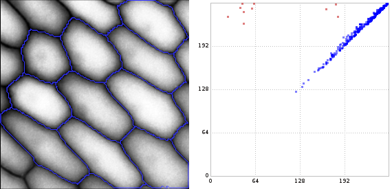
In the figure below, we see on the right the 1-dimensional persistence diagram computed by libstick and visualized by lyxtor². The red points in the diagram have been selected and visualized as blue cycles on the left.³ Seven of them are born in the interval [16, 64] and three of them are born in [160, 192]. (The latter three correspond to those onion cells that are a bit trimmed by the image boundaries.) The birth time of a cycle is the gray value of the brightest pixel of a cycle. The death time of a cycle is the gray value of the brightest pixel enclosed by it.

Merging components

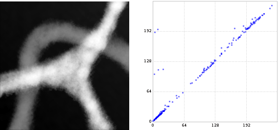
Below we see another gray-scale picture and the 0-dimensional persistence diagram of the sub-level set filtration. The picture shows a very bright star shape with three branches and a mid-gray path crossing two of the bright branches. The 0-dimensional persistence diagram reflects this: At a low level, we have 6 quite black components. As the level rises beyond the gray value of the mid-gray path, 3 components are merged with 3 others, causing three points in the diagram at about a gray value of 100. Later, when the level rises beyond the gray value of the star shape, the final three components are merged to a single one, causing the two points in the diagram at a gray value of about 192.