Voronoi diagram of a convex polyhedron

In this little blog article, we will show how the Voronoi diagram of a convex polyhedron \(P\) in \(d\)-dimensional Euclidean space can be computed in \(O(n^{\lceil \frac{d}{2} \rceil} + n \log n)\) time. As the attentive reader might guess by the time complexity, this is done by intersecting \(n\) half-spaces in \(\mathbb{R}^{d+1}\).

Preliminiaries. The Voronoi diagram of \(n\) sites¹ tessellates space into \(n\) so-called Voronoi cells, each of which consisting of those loci that are closer to the defining site than to any other. When we speak of the Voronoi diagram of a polyhedron \(P\), then we consider the set of faces of \(P\) as the set of sites. Also, we are here only interested in the Voronoi diagram within \(P\).² Below we see the Voronoi diagram (blue) of a polygon (black), i.e., a polyhedron in the plane:

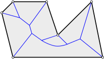
Each face of \(P\) has a Voronoi cell that is bounded by blue lines and its defining site (as we restricted the Voronoi diagram to \(P\)). The Voronoi diagram consists of loci that are equidistant to two sites. Hence, it is made of pieces of straight lines and parabolas in the plane, resp. quadrics in higher-dimensional space.

Convex polyhedra. The Voronoi cells of the convex vertices are collapsed to a point. This observation can be generalized:

Lemma. If \(P\) is a convex polyhedron³ then only its facets⁴ have Voronoi cells with non-empty interior.

Proof. Consider a point \(p\) in the interior of \(P\). It suffices to show that all closest⁵ faces of \(P\) to \(p\) are facets. Assume to the contrary that \(F\) is closest and \(i\)-dimensional, with \(0 \le i \le d-2\), and let \(r\) be the distance. Then the ball \(B\) centered at \(p\) and with radius \(r\) does not intersect \(P\) in its interior, but touches \(F\) in a point \(q\). Hence, a local neighborhood at \(q\) on \(P\) is contained in the tangential hyper-plane at \(q\) on \(B\). In other words, \(F\) is flat, which is a contradiction.

From this lemma it follows that we only need to consider the facets of \(P\) in order to determine its Voronoi diagram. A point \(p \in P\) belongs to the facet \(F\) that minimizes its orthogonal⁶ distance to \(p\). Let \(f_F \colon P \rightarrow [0, \infty), p \mapsto f_F(p)\) denote the orthogonal distance of \(p \in P\) to \(F\) and let \(f \colon P \rightarrow [0, \infty), p \mapsto \min_F f_F(p)\). The point \(p\) belongs to the Voronoi cell of \(F\) if \(f_F(p) = f(p)\). That is, the function graph of \(f\) is piecewise linear and projecting its faces onto \(P\) gives the set of Voronoi cells resp. the Voronoi diagram of \(P\). Also note that each Voronoi cell is a convex polyhedron itself.

Algorithm. Let us consider for each \(F\) the half-space \(H_F\) in \(\mathbb{R}^{d+1}\) that contains \(P\) and whose boundary supports the function graph of \(f_F\). Computing the function graph of \(f\) is equivalent to intersecting the half-spaces \(H_F\). Using duality between points and hyper-planes, the convex hull algorithm by Chazelle⁷ solves this problem in optimal \(O(n^{\lceil\frac{d}{2}\rceil} + n \log n)\) time.

Concluding remarks. As a side product, one obtains that the combinatorial size of the Voronoi diagram is at most \(O(n^{\lceil\frac{d}{2}\rceil})\). For convex polyhedra, the straight skeleton, Voronoi diagram and medial axis are equal. In fact, the above technique has already been applied to compute the straight skeleton in the plane by consider lower envelopes of (partially defined) linear functions. For straight skeletons of general input, however, the difficulty is to construct for each linear function its individual domain such that the lower envelope representation works out. For convex polygons, the domain becomes trivial, as illustrated above. Also, to compute the Voronoi diagram of points, Chazelle transforms the problem to intersecting half-spaces. In fact, it would not be too surprising, if the result mentioned above can be found somewhere in the literature. If you know of any reference, I would be glad if you could tell me.

I would like to thank Anna Lubiw for mentioning this problem.

Update. Anna Lubiw informed me that in a technical report Mitra and Hafer⁸ used basically the same technique to solve this problem.